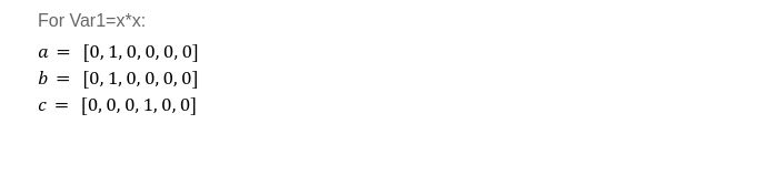
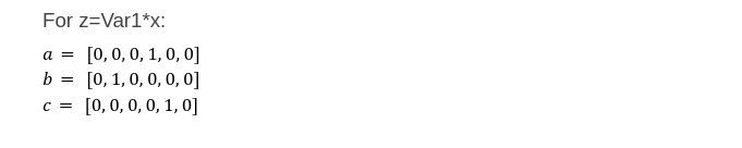
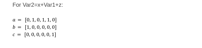
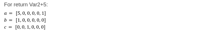
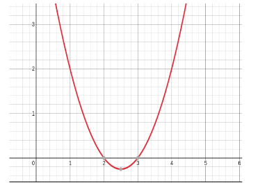
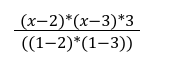
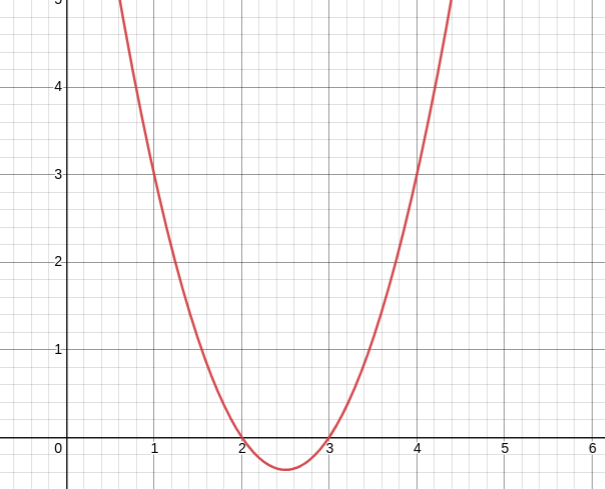
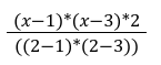
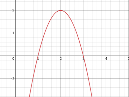
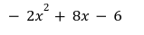
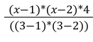
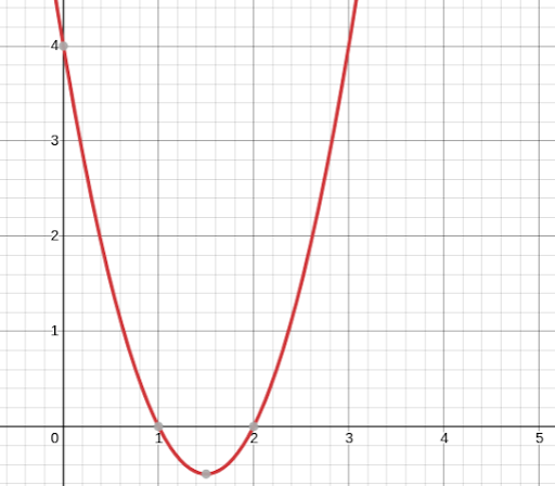
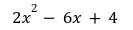
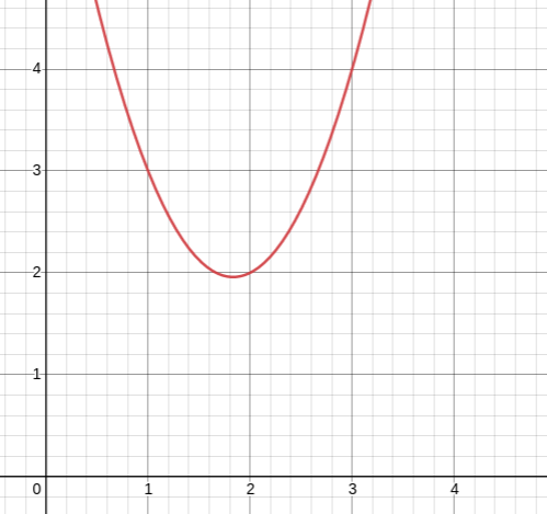
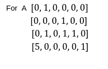
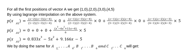
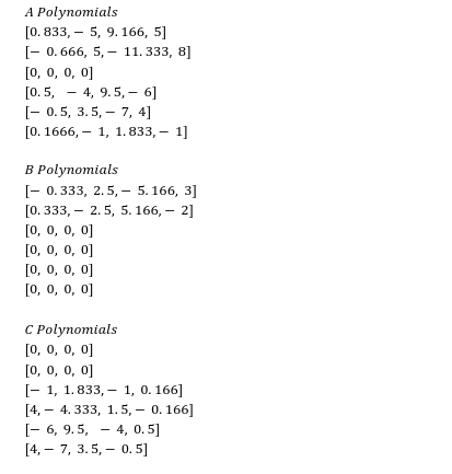
This article is greatly inspired by Vitalik explanation on Quadratic arithmetic programs(QAPs). In this article we are going to take a direct approach to understand the complex step in making snarks or you may say that the first step of representing the massive state data into a low degree polynomial. If you are not familiar with the basics of polynomials and what benefits do they really offer? you may refer to this article. To begin with, we must know that ZK-snarks are not applicable to any computational problem. There are few NP problems(such as boolean satisfiability) which are computationally infeasible to verify. When we say that every NP problem has zero-knowledge proof, what we mean is that any NP problem instance can be proven to be true in ZK. This is what Goldreich, Micali and Wigderson explained in their paper . So to operate the problem we first have to convert the problem into a right form. This form is termed as Quadratic Arithmetic Program. This step is separate and will run in parallel alongside the zero-knowledge proof creation and its verification. The flow of QAP is program→circuit→R1CS→QAP QAP is a process of transforming the code of a function into a mathematical representation which upon providing input to the code, delivers a corresponding solution. We are starting with a simple example The special purpose programming language which has been used here supports only the basic arithmetic operation such as (+,-,*,/) and constant exponentiation such as (x**7 not x**z). The comparison(<,>,==) and modulo (%) operator is not applicable here, though we can use the conditional statement in arithmetic form: For example: (if x>3: y=5 ; else y=4) can be written as : y=5*(x>3)+4*(x<=3). Now, we have the specifications, let's move towards the first step of conversion which is flattening. Flattening is the process where we convert the original code into a sequence of statements which are of two types. This is similar to the conversion of code into logic gates. Thus the result of flattening our code will look like this: Now in the next step we convert the flattening output to a system called R1CS. R1CS is a core concept of zk-SNARK which provides an easy verification format for zero-knowledge proofs. It simply assigns the result of multiplication or sum of variables into a new variable. This ensures that indeed the computation has been performed but in a different format. To read more on R1CS you can refer to this great article. There are three vectors (a,b,c), and a solution to R1CS is a vector s where s must satisfy the equation s.a*s.b-s.c=0 (the dot represents the dot product). The s is a witness vector which consists of all the values associated with the variables that have been used during the computation. We are using a standard way of converting the logic gate into (a,b,c) vectors depending upon the operations(+,-,*,/) and arguments(constants or variables). The length of each vector depends upon the total numbers of variables in the system including two dummy variables ~one (which at the first index representing 1) and ~out (representing output). This also includes input variables or public inputs (44), private input (x) and intermediate variables(z,var1,y). To move ahead, let's see the variable mapping we will use to represent the solution vector in the same order. The mapping here has significance which I am leaving for some other post. '~one', 'x' , 'out', 'var1' , 'z', 'var2' You can see from mapping that the vector a, b value is 1 only where the input x is enabled making it to x2 in vector c at var1 mapping. Similarly for the next gate: Here the pattern is little different: it's multiplying the first position of vector b with the second, fourth and fifth position of vector a and add them together to ensure that indeed the sum of these multiplications is the sixth element of vector c. Now finally for the fourth and last gate. Here in the last check the dot product checks the sixth element of vector a, adding five times the first element resulting 5 and checks it against the third element of vector c where we have stored the final output. With that we have successfully constructed the R1CS system with four constraints. The witness here is simply the assignment of private input x, public input 44 and other intermediate variables. s=[1, 3, 44, 9, 27, 39] Now combining the whole R1CS system together with these four gates, we get 3 vectors for 4x6. The last step is to convert the R1CS into QAP with the same logic on polynomials instead of Dot product. We will transform the system of four groups of three vectors of length six, into six groups of 3 degree polynomials, where evaluating the polynomials at each x coordinate represent a constraint. How do we do that? Lets see this short example first. For polynomials we often use lagrange interpolation. Suppose you have a set of points (1,3),(2,2),(3,4) and you want to find a polynomial which passes through all these points. We could achieve this by lagrange interpolation. To start with point (1,3) we will make the y component 0 for the other coordinates of x such as (2,0),(3,0). Now for the equation (x-2)(x-3) we have a graph: We can see that at x=1 the height is not what we desire. So to adjust that we have the equation below: This gives us the below graph: We then do the same by sticking at the point x=2 and x=3: For x=2: This gives us: Similarly for x=3 we have: Now adding all three together we get: So now, the same strategy will apply to our R1CS system. What we are gonna do is to take the first value of every vector a, apply lagrange interpolation to make a polynomial for it. We then will repeat the same process for vectors b and c. We will also apply the same methods on vector's second values, third values and so on. For all the first positions of vector A we get (1,0),(2,0),(3,0),(4,5). By using lagrange interpolation on the above system. Evaluating these polynomials at x=1 will give us the set of vectors for the first logic gate that we have created. If the equation s.a*s.b-s.c gives a non-zero value, that means atleast one of the x representing a logic gate gives a non-zero value which emphasizes that the values goes in and out of the circuit are inconsistent. We are leaving the further concepts and machinery of snarks for another post. From here you can also read about zero-knowledge proofs.Quadratic Arithmetic Program
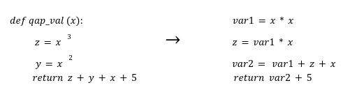
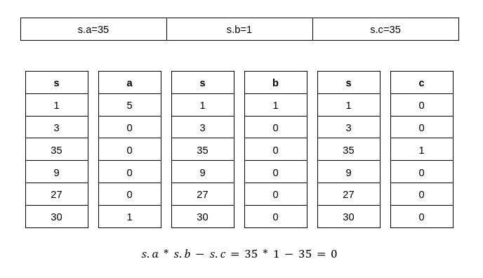
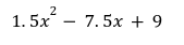
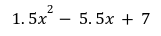
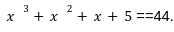 Now, let's get started with the steps of QAPs. We can define the function of the given equation as:
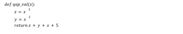
Flattening
Rank-1 Constraint System
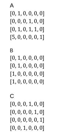
R1CS to QAP
Example:

We develop cutting-edge products for the Web3 ecosystem supported by our extensive research on blockchain core and infrastructure.

