Polynomial Commitments For Stateless Clients

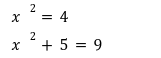
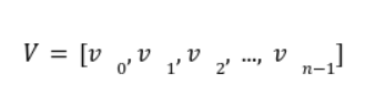
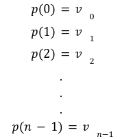
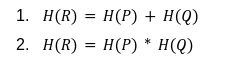
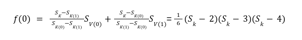
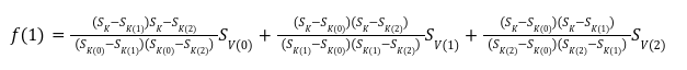
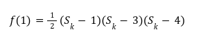
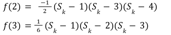
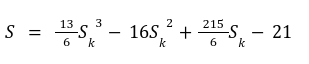
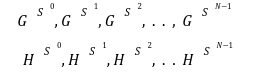
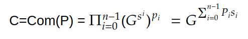
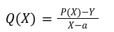
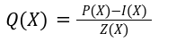
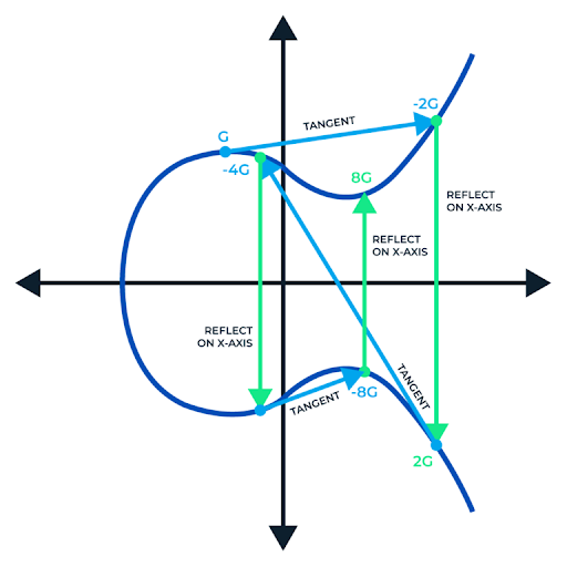
In our previous article we have described what stateless clients are, why they are important and how we can achieve statelessness in Ethereum. However we have seen that the witness required for validation has a huge size which must be addressed before moving further. So here we are presenting “Polynomial Commitments” as a possible solution to the above mentioned problem.

The current blockchain state is nothing but a vector space. It stores data in the form of vectors. The three kind of vectors it stores are:

1. Vector for account keys - 32 bytes.
2. Vector for account values - 128 bytes(includes nonce, balance, byte code, storage root).
3. Vector for storage values - 32 bytes.

The storage vector itself gets included into the root hash. For this, we don't need to explicitly consider this while forming a polynomial. So we only need two polynomials for the state. Before we get into creating a polynomial, let's find out the unique characteristics held by polynomial commitments.

What are Polynomial Commitments?

A polynomial commitment is a commitment hash of 32 bytes representing some polynomial P(x) with the ability to perform arithmetic operations on hashes. In a typical polynomial commitment, the Merkle roots have been replaced by a mathematical representation called polynomial commitments. 

For example, given a starting point x, compute that

and repeat it for 1 million nodes. The ultimate goal is to prove that I have computed it correctly without the other node to re-run the whole thing.

Let's say i start with x=2.

So my trace would be {2,4,9,..}.

Now to do it again and again for 1 million nodes will publish a vast amount of data. How can I convince the verifier that I have computed this? Well, I could commit to some piece of data which is a digest to all these million numbers. This could be done in a way that you, the verifier, can ask me to evaluate at some random points and verify my evaluation. It has the following advantages.

1. Polynomial commitments take less computation to compute complicated proofs due to their mathematical structure.
2. It is a scheme that allows cryptographers to load large amounts of data into a single point on an elliptic curve. 
3. Polynomial commitment schemes use a polynomial which behaves like a vector space where each dimension(or term) is loaded with data which is separated mathematically E.g (3X²+6X+2).

For a vector

 the polynomial P(x) will give:

Note here that in a Merkle tree, the hashes of child nodes can not be added to form the hash of the parent node. However, in the polynomial commitment, we can perform arithmetic operations on hashes. For example, given three polynomials hashes we have, H(P)=Commit(H(P)), H(Q)=Commit(H(Q)) and H(R)=Commit(H(R)) on three polynomials H(P) ,H(Q), and H(R).We can verify the following modulo equation[1] (Why we use modulo math we will see later in this article).

Creating A Polynomial From Vector

Let’s assume that we are trying to store the state as two polynomials instead of a Merkle tree.  The two polynomials are S_K(X) and S_V(X). The S_K(1), . . . S_k(N) represent the public keys while the S_V(1), . . . S_V(N) represents the account values corresponding to those keys. So let's suppose we have accounts S_K(0)= 1 , S_K(1)= 2 , S_K(2)= 3 , S_K(3)= 5  and values representing to these corresponding account are S_V(0)= 1 , S_V(1)= 4, S_V(2)= 1 , S_V(3)= 5 therefore the general form of Langrange polynomial interpolation for the given function is :

Similarly for other values, we get the following functions:

Adding all the values of the above function we get the following value for s.

Committing To A Polynomial

Let G₁and G₂ be the two elliptic curves with a bilinear pairing e: G1×G2→GT and p is the order of G₁and G₂ whose generators are G and H correspondingly.

The trusted setup has created a reference string or public parameters with the use of a secret s. This secret s is unknown and can never be known by anyone; however, the public parameters will be known by each node. Using multi-party computation one can agree on a secret s and anyone can compute these public parameters easily. 

The G is an individual point, with two coordinates x and y so the entire commitment will be one group element.

Note: This is computationally infeasible to know the secret s from public parameters.

So now we have a polynomial P(X)=P₀X₀+P₁X₁+ . . . +P_n-1X_n-1 and we want to commit this polynomial .

 The ∏ will perform the dot operation.

Evaluating Polynomial

Suppose we have a sequence of values as vector V=[v₀,v₁,v₂, ..., v_n-1] and we have turned this vector into a polynomial P(X)  using lagrange interpolation such that P(i)=v_i.So if a verifier asks to evaluate P(a)=y_i, the prover needs to compute Quotient polynomial:

The above equation holds the same relation as the equation below:

• The I(X) is nothing but the evaluation of a polynomial at multiple places of D. where D is the data which evaluates to the value y_i at position z_i.

D=(z_o,y_o),(z₁,y₁),(z₂,y₂), . . . (z_n-1,y_k-1)

• The Z(X) or zero polynomial is a polynomial which is equal to zero at X=x₁+x2+, , ,+x_n-1.

Z(X)=(X-z₀),(X-z₁),(X-z₂), . . . (X-z_k-1)

Z(X) is used for the verification of commitment that is C if it is a commitment to polynomial P(x) created with the information D. If the case is true the output will be 1 otherwise 0.

The quotient polynomial Q(X) implies that P(X)-Y is a multiple of Z(X). hence that  P(X)-I(X) is zero where Z(X)=0. So the prover will form a polynomial Q(X) which deducts the original polynomial P(X) from the evaluated polynomial I(X) and divides it to zero polynomial Z(X). 

Now keeping the structure in mind let's draw an image that conforms to the evaluation of Q(X). 

The Prover Work

1. State→vector→polynomial→polynomial commitment C (The client will only store this commitment).
2. State data is D, the prover will compute Z(X), I(X) and Q(X).
3. The prover then turn the quotient polynomial Q(X) into a commitment π(proof).
4. The prover then broadcast the block along with witness (D,π).

The Verifier Work

1. The verifier will get the block along with (D,π).
2. He will then recompute the Z(X) and I(X) from some points.
3. Commit Z(X) →Z, I(X)→I.

Checks C-I=Zπ. (The commitment C is common to both for prover and verifier).

Verifying Using Pairing

With reference to this equation where the verifier needs to prove:  C-I=Zπ. To prove this the verifier needs to use a pairing method.

But why are we even using pairings? What is the exact reason behind this? Well to know about this we first need to know how the elliptic curve behaves.

Elliptic curve is an asymmetric cryptography based on discrete logarithm which is expressed by the addition and multiplication of points on the elliptic curve.

This curve lies on a finite field p which creates this illusion of dots scattered in two dimensions. The elliptic curve in cryptography deals with extremely large numbers of computing over a finite field. We know that while using finite fields we apply modulo arithmetics operations to withhold its properties(such as commutative and associative). 

The elliptic curve[2] and finite fields[3] are greatly demonstrated in these references.

The field behaves fine while performing addition and subtraction but when it comes to multiplication the curve points may lead to infinity. 

As we have discussed above the verifier needs to perform multiplication while proving the commitment so for this purpose the concept of pairing has been introduced which states that:

A bilinear map from G₁×G₂→G_T is a function

e: G1×G2→GT such that for all u∈ G1,v∈G2 , a,b∈ Z

e(u_a, v_b)= e(u,v)^_ab

So we can rewrite this equation C-I=Zπ as e(C-I-H)=e(π,Z)

The H here is the generator for G₂ group which translates the term C-I into G_T.

So should we continue to store the state as a polynomial commitment for witness size compression? Maybe not because the above technique has arisen two significant problems.

1. We have 2^₃₀ state size, so generating a witness for N keys will still take the output time of O(dlog^2d+nlogn) where n is the state's size, which is approximately equal to 2³⁰or 50 GB. This considerable size has made the technique impractical to generate such huge proofs within a single block.
2. Updating the digest, for example, the values of S_K(x) and S_V(x)will also take a huge time. 

References

1. Modulo operation
2. Ace addresses and signatures with bitcoin
3. Learning cryptography finite fields

You can also read on our latest publication on Curve Cryptopools.