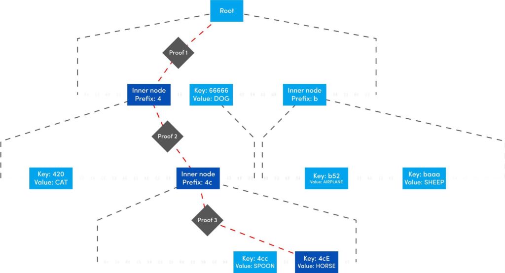
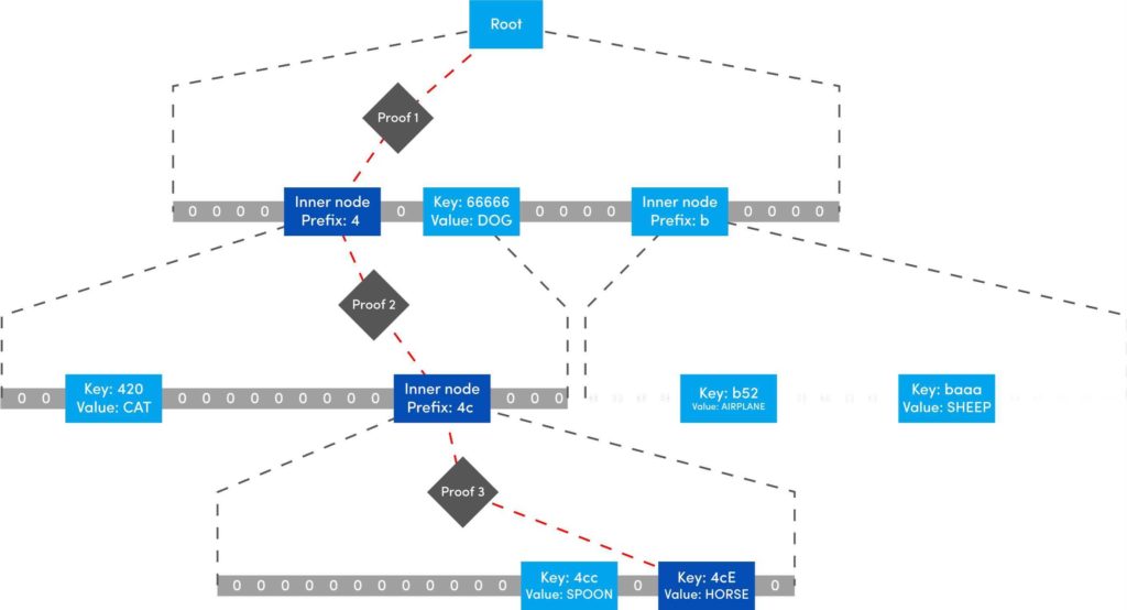
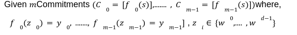
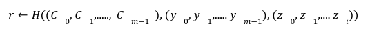
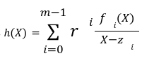
This is the last post of our series on stateless Ethereum. Earlier, in the previous articles we have discussed the concept of stateless clients and its necessity in serenity. We have also discussed Kate commitments as a commitment scheme under polynomial commitments. Now, before moving further lets comprehend the origination of “Verkle Trees”. You might be thinking what Verkle trees are. Well, this is one of the solutions proposed for Ethereum’s scaling upgrades which is the efficient replacement of “Merkle Trees”. Verkle trees were first introduced by John Kuszamaul[1] in 2018. It is a data structure which combines the magic of trees and cryptographic accumulators. They can store a large amount of data and generate a short proof of it, which could easily be verified by anyone who has the root of the tree. Verkle trees use the mathematical construction of Kate commitments where each node has a width of 256. Sounds difficult? Well don’t worry we will understand the above statement thoroughly in this article. But first let's see what are the few differences we have in comparison to Merkle trees: Suppose you want to reach the position 4cE. So to acquire the proof you must include all the sister nodes highlighted in light blue at each level until we reach the root hash which is quite bizarre. On the other hand, In Verkle tree we do not have to provide all the sister nodes instead, we just provide the path with a proof. This is the main reason why the Verkle tree drives a huge benefit from greater width and leads to shorter paths. Assume that we have randomly distributed values here. So the path goes down from top to a particular value will take the log256(n) time. So the problem is, if we use the regular hash function to generate the proof with the width of 256 it will produce a huge size of witness. This is why we use Kate commitment for these nodes instead of using roots as the hashes. To understand this, we first need to know that a typical hash function which computes the hash of a parent node from its children is not a regular hash, but a vector commitment. A vector commitment scheme uses a hash function which takes a hashing list h(v1,v2,v3,...)→C. These vector commitments can create a short proof that commits to some list. In the Verkle tree these short proofs are the efficient replacements of child nodes hashes as given below in the image. In practice, instead of using vector commitments,we use a more powerful approach to create these proofs which are polynomial commitments. This is because polynomial commitments let you hash a polynomial and make a proof for the evaluation at any given point. To learn about more on polynomial commitments read this article[2]. This article is greatly inspired by the maths explained by Dankrad Fiest in his article[3]. This article is the simplest form of maths which combines the dynamics of verkle trees and polynomial commitments. There are multiple polynomial commitments schemes available which provide flexibility and efficiency. Out of which the one which is easiest to use is KZG commitments[4]. Kate commitment is a polynomial scheme which uses elliptic curves pairings[5] and polynomial maths to create a data structure which can include any value upto 256. But here comes the exciting part. This inclusion of the values can be proven by a single witness. Multi-Proofs are the proofs that are generated for multiple key/value pairs at the same time. Multi-Proofs with kate commitment states that: given M commitments and N leaves spread across those commitments, you can make a single proof which is less than 200-bytes. To begin with Multi-Proofs with PCs let's get the example below. Consider you want to prove the leaf value 0101 0111 1010 1111213. To reach the index 1010 highlighted with blue you need to provide commitment to Node A and Node B along with the proof at each level. You need to prove that: We assign the commitments to Node B→C0 , Node A→C1 and Root →C2 into a polynomial function fi(X). This implies that the function fi(X)is committed to Ci ,which evaluates y_i at some index zi. For example: fi(zi)=yi. Hence, You might be wondering why we haven't used simple zi in the parameter of function. Well, this is because we are using elliptic curve pairing which performs modulo arithmetic operations. So in order to make our field finite we are using the extension field where w is the dth- root of unity which makes operations more efficient. where, Note here that if we want to go deeper in the tree to access the node, the size of the multi-Proof will be increased. So we end up with thousands of evaluations at The Verkle multi-Proof must validate the following relation: Instead we take one proof for each commitment along the path of the node, we use the exceptional properties of polynomial commitments to make a single fixed size proof which validates all parent-child links along the path for greater number of key/value pairs. For each node we need to provide that the next coming node is actually the child of the above node. The greater the nodes, the greater the linkages. Let r belong to the hashes of commitment, some value and index. The prover computes the equation: To prove that the g(X)is the real polynomial, the quotients of the equations must be exact divisions. This is because if we add the quotients, the results should be canceled and we have a polynomial not a rational function. Now any function we commit using a Kate commitment is a polynomial. The prover computes the polynomial and sends the commitment C=[g(s)] to the verifier. This commitment should convince the verifier that the indeed it is the commitment of the function g(X).The g(X) term is only computable if that expression is a polynomial not a fraction. Thinking about how it works? Let’s get into it with a low degree example. Moving to the next section we are going to understand the step by step process for the polynomial to commit by the prover, and verify by the verifier. To prove that C_i the real commitment to polynomial g(X).We need to follow two things. We will do this by evaluating the polynomial at an equation. Using mathematical rules we can split the sum: The prover computes The term The Opening, The commitment O can be verified by the verifier using a multi-exponentiation method. The Evaluation must satisfy the condition O=h(X). Let The verifier can easily computer the term The proof consist of and C. The verifier can verify the proof using the following equation: This shows that the commitment C opened at any random point(The prover has no idea about this random point while committing to the polynomial) is exactly equal to g(t)which the verifier has computed with the help of a prover. Hence the proof is complete. The goal of Stateless clients is to make Ethereum stateless and bring cheap consensus nodes. Though the Ethereum community has provided us with various possible solutions for stateless clients, the fire of research is still burning.Verkle Trees
Why Not Regular Hash Function?
Vector Commitments
Polynomial Commitments and Multi-Proofs
Kate Commitment
Multi-Proofs

![]()
![]()
The Relation to Prove

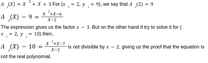
Step1: Evaluation of A Polynomial
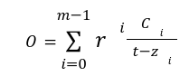
The Prover
 because the function f_i is only known to the prover.
The Verifier
![]() is completely known by the verifier and can be computed easily. However for
is completely known by the verifier and can be computed easily. However for ![]() The verifier is provided by an opening by the prover. Here the prover provides the commitment
The verifier is provided by an opening by the prover. Here the prover provides the commitment 
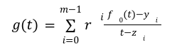
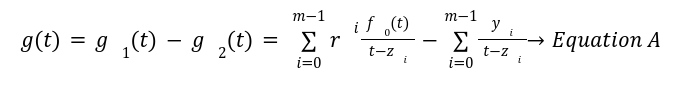
Step2: The Proof
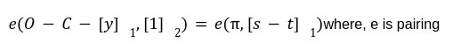
![]() be the polynomial committed by C. So if the prover is honest, then this will be the g(X). To conclude the proof the verifier needs to check:
be the polynomial committed by C. So if the prover is honest, then this will be the g(X). To conclude the proof the verifier needs to check: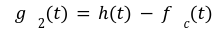
![]() from the equation A while, the other two terms are provided by the prover to the verifier. So the KGZ proof will be :
from the equation A while, the other two terms are provided by the prover to the verifier. So the KGZ proof will be :
Step3: Verification of Proof
Conclusion
References

We develop cutting-edge products for the Web3 ecosystem supported by our extensive research on blockchain core and infrastructure.

