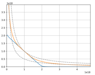
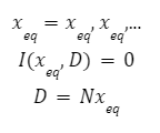
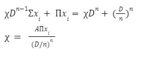
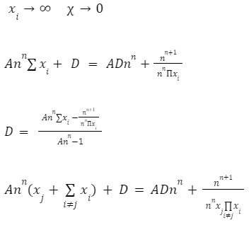
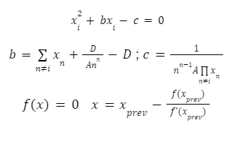
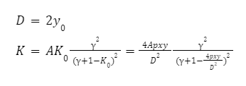
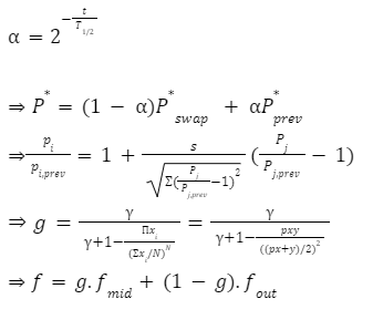
The automated market makers are the main protocols of the decentralized exchanges that were first introduced by Uniswap. They introduced the concept of the product linear invariant. Which has the sole motive to spread liquidity evenly other than the pricing of the underlying assets. Later stableswap came up with the new idea of AMM which introduced the concept of stablecoin-to-stablecoin trading and spreading the liquidity evenly while maintaining the price of both flavors. In the new version of the curve they have introduced the method where liquidity is spread by internal oracles, for the assets that are not pegged. But the prices here are only changed when the ratio of loss is small as compared to the profit that is generated by the system. This results in the increase of liquidity by 5 to 10 times as compared to uniswap. You can learn about stableswap in this article . In this AMM model we adopted the method of linear transformation and we span them around the targeted value of 1. This method is already being followed in ypool and compound pool which allows us to preserve the structure. Here we suppose balances in smart contract as the vector presented as b=(b0, b1,.....)where bi is stated as the balance of i-th token and the price scale p= (p0, p1,..) is the coefficient of the balance b. Therefore we transform the b into b’ and hence it can be written as Where the invariant is represented into the form of 2-dimensional hypersurface. In the above the orange line represents the line that is obtained by the above calculation we can see that it is more stable then the constant-product invariant (dashed line) and the stableswap is represented in blue line Here the identity transformation is We suppose that the the 0-th asset in the pool is USD and the price p0=1the invariants are constructed in such a way that when their identities are transformed they transform at 0 We can say that the above designed curve depends on the tokens deposited in the pool therefore we introduce a new variable D which is the sum of all the tokens in an equilibrium pool. We can write as Where D is the sum of all the tokens that are pegged and thus the above solution gives us a trivial solution. In stableswap invariant we have seen that they have joined both the Constant product invariant and Constant Sum Invariant in order to achieve the lower slippage cost. Moreover we introduced a constant which depends on the number of tokens deposited in the pool and multiplied with the CSMM. at equilibrium at equilibrium at imbalance Let us consider an ideal case where the number of each token in the pool is the same. Hence the equation gives us a trivial solution at the equilibrium. We know that chi is the weight and D^n-1is multiplied to make the CSMM and CPMM of same magnitude. However the case is not same when pools are not in equilibrium and is a constant number then the equation is n longer valid. Therefore we made dynamic that is when the pools are in extreme imbalance conditions the limit extends to zero resulting constant product variant dominant. Where as is kept equal to A in an equilibrium condition which helps us to hold the condition at all the time. Now let's look at how stableswap derives the swaps outcomes. Continuing with above equations and number of tokens in the pool we can calculate D. For example if we want trade token i we can separate xi and solve the equation with respective to xi Since the vyper language can not compute quadratic equations therefore we use Newton's iterative method. The above formula doubles the precision with every iteration which helps to calculate a suitable amount of gas limit. Lastly the difference between xi before and after states the amount of i tokens bought. Where K0 varies between the values of 0 and 1 1 = equilibrium pool Below is the graph of and K as function of K0: Here we can see that as the value of y drops the AMM reacts more as CPMM even though the pool is only a little bit imbalanced. Which indicates a drastic change in the price .The Curve V2 also focuses on how to control such drastic price transitions. Therefore we consider that an equilibrium point on the market hence the equation becomes. The above function can be written in the terms of A, y, p D, x, y. The function can be written as a cubic function as shown below. The Curve V2 achieves a very small amount of slippage when compared CPMM and as long as price pegs are considered we change p in cubic form in the equation above hence the problem is solved. In order to calculate the swap results we can again use Newton's method to find the amount of desired token bought out. In order to be sure about our gas limit curve, the whitepaper discusses the starting assumptions and the parameters of the function, where they have used a method named fuzzy (hypothesis framework) about which much knowledge is not known. To keep the slippage as least as possible Curve V2 constantly fixes the market maker function by adjusting the price scale. Here Curve V2 introduces a new variable named Xcp which adjusts the losses gained by liquidity providers. Which is defined as If the loss occurs after one repegging then the algorithm will keep the market maker function the same. This version of Curve uses the internal oracles that help to determine the oracle price and maintain the price according to the market, these oracles use exponential moving average. Here we introduce a new vector named price oracle that is linearly independent. They lag the price behind the oracle price by introducing the new vector s. This equation can easily be derived using Euclidean geometry. The variables here EMA price oracle and price scale reduces the drastic changes in the price and represents a long term steady price. Due to the market maker feature of Curve V2 discussed above, we can say that it is better to make transaction fee a linear combination of 2 tiers of transaction fees with the dynamic weights measuring the distance from the equilibrium point. The f-mid and f-out value is decided by the Curve V2 and it is kept at 0.04% and 0.4% respectively. The market maker function can be pegged to any price instead of stablecoin. The transition of the price is much smoother than the stableswap. And the prices are constantly being monitored and updated with the help of an internal oracle. Which allows the user to trade in an equilibrium market. However on the other hand if we look mathematically the model can result in suggesting higher gas prices due to the cubic equation. Curve V2 and stableswap both have the aim to minimize the slippage as low as possible however curve V2 has focused more to peg the assets with the current market price. I would like to acknowledge and give my warmest thanks to Shakieb Shaida. Who made this work possible.for letting my defense be an enjoyable moment, and for your brilliant comments and suggestions, thanks to you. You can also read upon our latest publication on Amphora: The Merge EventIntroduction:
Using Linear Transformation for pegged invariants:



Curve Crypto-pool AMM:



To ensure a more smooth price changes Curve changes chi its dynamic weight to K as shown below: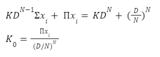

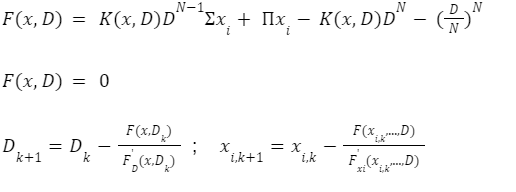
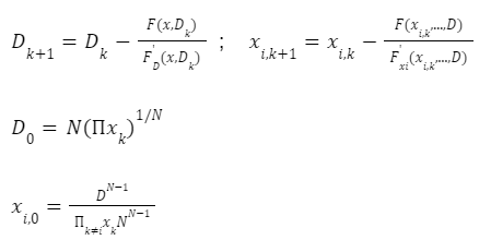
Here
0 = imbalance pool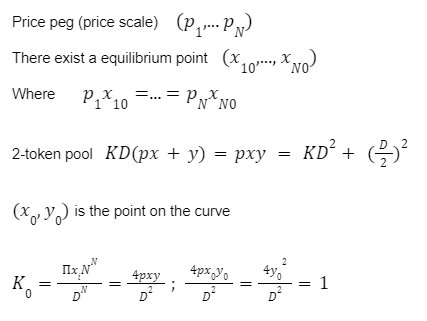


Repegging Algorithm:
Discussion:
Conclusion:
Acknowledgment:
References:


